
Chapter 21 of 163 · Man, Economy, and State, with Power and Market by Murray N. Rothbard
6. Elasticity of Demand26
The demand schedule tells us how many units of the purchase good will be bought at each hypothetical price. From this schedule we may easily find the total number of units of the sale good that will be expended at each price. Thus, from Table 2, we find that at a price of 95, three horses will be demanded. If three horses are demanded at a price of 95 barrels of fish, then the total number of units of the sale good that will be offered in exchange will be 3 × 95, or 285 barrels of fish. This, then, is the total outlay of the sale good that will be offered on the market at that price.
The total outlay of the sale good at each hypothetical price is shown in Table 3.
TABLE 3
| BUYERS | ||
|---|---|---|
| PRICE | DEMANDED | TOTAL OUTLAY SALE GOOD |
| 80 | 9 horses | 720 barrels of fish |
| 81 | 9 | 729 |
| 82 | 9 | 738 |
| 83 | 9 | 747 |
| 84 | 8 | 672 |
| 85 | 8 | 680 |
| 86 | 7 | 602 |
| 87 | 6 | 522 |
| 88 | 6 | 528 |
| 89 | 5 | 445 |
| 90 | 4 | 360 |
| 91 | 4 | 364 |
| 92 | 3 | 276 |
| 93 | 3 | 279 |
| 94 | 3 | 282 |
| 95 | 3 | 285 |
| 96 | 2 | 192 |
| 97 | 2 | 194 |
| 98 | 2 | 196 |
| 99 | 1 | 99 |
| 100 | 1 | 100 |
| 101 | 0 | 0 |
Figure 17 is a graphic presentation of the total outlay curve. It is evident that this is a logical derivation from the demand curve and that therefore it too is a curve of outlay by buyers at each hypothetical price.
A striking feature of the total outlay curve is that, in contrast to the other curves (such as the demand curve), it can slope in either direction as the price increases or decreases. The possibility of a slope in either direction stems from the operation of the two factors determining the position of the curve. Outlay = Price × Quantity Demanded (of purchase good). But we know that as the price decreases, the demand must either increase or remain the same. Therefore, a decrease in price tends to be counteracted by an increase in quantity, and, as a result, the total outlay of the sale good may either increase or decrease as the price changes.
For any two prices, we may compare the total outlay of the sale good that will be expended by buyers. If the lower price yields a greater total outlay than the higher price, the total outlay curve is defined as being elastic over that range. If the lower price yields a lower total outlay than the higher price, then the curve is inelastic over that range.
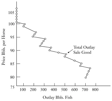
FIGURE 17. TOTAL OUTLAY CURVE
Alternatively, we may say that the former case is that of an elasticity greater than unity, the latter of an elasticity less than unity, and the case where the total outlay is the same for the two prices is one of unit elasticity, or elasticity equal to one. Since numerical precision in the concept of elasticity is not important, we may simply use the terms “inelastic,” “elastic,” and (for the last case) “neutral.”
Some examples will clarify these concepts. Thus, suppose that we examine the total outlay schedule at prices of 96 and 95. At 96, the total outlay is 192 barrels; at 95, it is 285 barrels. The outlay is greater at the lower price, and hence the outlay schedule is elastic in this range. On the other hand, let us take the prices 95 and 94. At 94, the outlay is 282. Consequently, the schedule here is inelastic. It is evident that there is a simple geometrical device for deciding whether or not the demand curve is elastic or inelastic between two hypothetical prices: if the outlay curve is further to the right at the lower price, the demand curve is elastic; if further to the left, the latter is inelastic.
There is no reason why the concept of elasticity must be confined to two prices next to each other. Any two prices on the schedule may be compared. It is evident that an examination of the entire outlay curve demonstrates that the foregoing demand curve is basically elastic. It is elastic over most of its range, with the exception of a few small gaps. If we compare any two rather widely spaced prices, it is evident that the outlay is less at the higher price. If the price is high enough, the demand for any good will dwindle to zero, and therefore the outlay will dwindle to zero.
Of particular interest is the elasticity of the demand curve at the equilibrium price. Going up a step to the price of 90, the curve is clearly elastic—total outlay is less at the higher price. Going down a step to 88, the curve is also elastic. This particular demand curve is elastic in the neighborhood of the equilibrium price. Other demand curves, of course, could possibly be inelastic at their equilibrium price.
Contrary to what might be thought at first, the concept of “elasticity of supply” is not a meaningful one, as is “elasticity of demand.” If we multiply the quantity supplied at each price by the price, we obtain the number of barrels of fish (the sale good) which the sellers will demand in exchange. It will easily be seen, however, that this quantity always increases as the price increases, and vice versa. At 82 it is 82, at 84 it is 168, at 88 it is 352, etc. The reason is that its other determinant, quantity supplied, changes in the same direction as the price, not in the inverse direction as does quantity demanded. As a result, supply is always “elastic,” and the concept is an uninteresting one.27
Man, Economy, and State, with Power and Market
Read the whole book online · Book details
Free to read online and to download from this archive.